Building Lattice Reduction (LLL) Intuition

The Lenstra–Lenstra–Lovász (LLL) algorithm is an algorithm that efficiently transforms a “bad” basis for a lattice L into a “pretty good” basis for the same lattice. This transformation of a bad basis into a better basis is known as lattice reduction, and it has useful applications. For example, there is attack against ECDSA implementations that leverage biased RNGs that can lead to private key recovery. However, my experience learning why LLL works has been pretty rough. Most material covering LLL seems targeted towards mathematicians and I had to (I guess I wanted to) spend a lot of time trying to weasel out the intuition and mechanics of the algorithm. This blog post is a semi-organized brain dump of that process. My goal is to cover LLL in such a way that slowly ratchets down the hand-waving, so feel free to read until you are happy with your level of understanding.

As an aside: if I'm wrong anywhere, please correct me! Hitting a nice balance of mathematical accuracy and intuition is tough, but I don't aim to be blatantly wrong. Please feel free to tweet at me if I screwed up. Its super possible I did.

Suggested Background

I don't think LLL will make much sense if you don't have a decent grasp on (at least):

• vector spaces and bases

• what a lattice is

• why lattice basis reduction is useful

• vector projections and the Gram-Schmidt process

I wrote another blog post on lattices and how they can be used to form an asymmetric cryptosystem. I think it would be a good thing to read first as it covers some of the suggested background.

LLL In-Relation to Euclid's Algorithm

LLL often gets compared to Euclid's Algorithm for finding GCDs . This is an imperfect analogy, but at a high-level they have a core similarity. Namely, both LLL and Euclid's algorithm could be broken down into two steps: “reduction” and “swap”. To illustrate consider the following pseudocode for both algorithms:

def euclid_gcd(a, b):
    if b == 0: # base case
        return a
    x = a mod b # reduction step
    return euclid_gcd(b, x) # swap step

# dont try to grok this yet...
def lll(basis):
    while k <= n:
        for j in reverse(range(k-1, 0)): # reduction step loop
            m = mu(k,j)
            basis[k] = basis[k] - mu*basis[j] # vector reduction
            # update orthogonalized basis
    if lovasz_condition:
        k += 1
    else:
        basis[k], basis[k+1] = basis[k+1], basis[k] # swap step
        # update orthogonalized basis
        k = max(k-1,1)
    return basis

If you squint a bit you can see the similarities in the pseudocode, but I think the core idea is that both algorithms use a reduce-and-then-swap technique to achieve their goals. So at this point, we can roughly say that LLL is an extension of Euclid's algorithm that applies to a set of n-vectors instead of integers.

Personally, I don't find that explanation to be satisfying but I can see why it could be a useful in developing understanding.

LLL In-Relation to Gram-Schmidt

Another algorithm that is similar to LLL is the Gram-Schmidt orthogonalization process. At a high-level, Gram-Schmidt (GS) takes in an input basis for a vector space and returns an orthogonalized (i.e. all vectors in the basis are orthogonal to one another) basis that spans the same space. It does this by leveraging vector projections to “decompose” each vector into related components and removing redundant components from all vectors. If GS doesn't make too much sense to you, I suggest checking it out before going too much further in this post. Not only is the algorithm similar to LLL, but LLL uses Gram-Schmidt as a subroutine.

You may say: “Why don't we use GS to reduce our lattice basis?” and we cant because life sucks sometimes. GS may get us closer to the basis we want, but GS is not guaranteed to produce orthogonal vectors that form a basis for our lattice. Check it:

sage: from mage import matrix_utils # https://github.com/kelbyludwig/mage; use the install.sh script to install
sage: b1 = vector(ZZ, [3,5])
sage: b2 = vector(ZZ, [8,3])
sage: B  = Matrix(ZZ, [b1,b2])
sage: Br,_ = B.gram_schmidt()
sage: pplot = matrix_utils.plot_2d_lattice(B[0], B[1])
sage: pplot += plot(Br[0], color='grey', linestyle='-.', legend_label='unmodified', legend_color='blue')
sage: pplot += plot(Br[1], color='grey', linestyle='-.', legend_label='orthogonalized', legend_color='grey')
sage: pplot

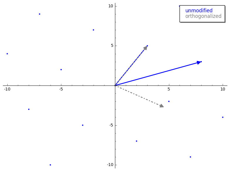
Notice how not all orthogonalized (grey) vectors are touching a lattice “point”? Fortunately for us, GS is still pretty useful to understanding LLL so this is not a total loss.

LLL In-Relation to Gaussian Lattice Reduction

Unless you are basically a sorceress, I imagine you may find starting with 2-dimensional lattice basis reduction useful. Thankfully, we have Gauss’ algorithm for reducing bases in dimension 2 . This is great for a couple reasons:

• Gaussian lattice reduction is also pretty similar to LLL

• Gaussian lattice reduction is analogous to both Euclid's algorithm and LLL so it can act as a bridge between these two analogies

• We can use 2D vectors which are easy to graph and visualize

Gauss’ algorithm is defined as follows:

def gauss_reduction(v1, v2):
    while True:
        if v2.norm() < v1.norm():
            v1, v2 = v2, v1 # swap step
        m = round( (v1 * v2) / (v1 * v1) )
        if m == 0:
            return (v1, v2)
        v2 = v2 - m*v1 # reduction step

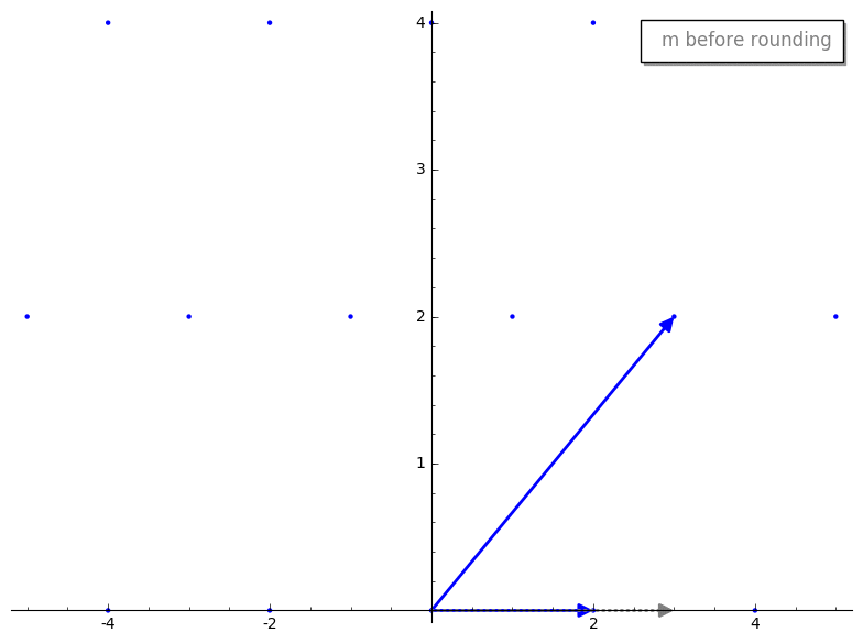
Let's break this down a bit. gauss_reduction takes in two vectors that represent our lattice basis. Ignoring the while loop for a second, the first step is the swap step. The swap step ensures that the length of v1 is smaller than v2. Among other things, this will ensure that the result of gauss_reduction will be ordered according to length which helps with some of the proofs that ensure this algorithm works well.

What does m represent? m is the scalar projection of v2 onto v1 (the longer vector onto the shorter vector). This is the same scalar produced during the GS process but in Gauss's algorithm we round it to the nearest integer so we ensure we are still working with vectors within the lattice. This is a important idea, so lets visualize this process.

We first project v2 onto v1. Here is what the projected vector looks like before and after rounding.

We then compute our new reduced vector v2 - m*v1. Here is the reduction step before and after rounding m.

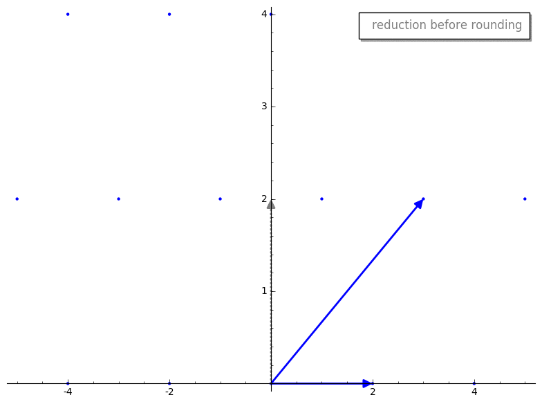
Cool, huh? By rounding m prior to reduction we have sorta “knocked over” our new reduced vector v2 so it becomes a vector in the basis. What is interesting is that the reduced v2 appears to have a shorter length than original v2. That is not a coincidence, that is a guarantee of the reduction step! Additionally, the resultant basis vectors will be “nearly” orthogonal, which is exactly what we want. I don't want to bog anyone down with details for why this works just yet, but if you are impatient you can jump to the more technical explanations .

For now, lets just wave our hands and say gauss_reduction will terminate, and return a “good” (i.e. short and nearly orthogonal) basis for dimension 2 bases.

LLL tl;dr

LLL extends Gauss’ algorithm for reduction to work with n vectors. At a high-level, LLL iterates through the input basis vectors and performs a length reduction to each vector (this is close to Gauss’ algorithm at this point). However, we are dealing with n vectors instead of just two so we need a way to ensure that the ordering of the input basis doesn't affect our result . To assist with ordering the reduced basis by length, LLL uses a heuristic called the Lovász condition to determine if vectors in the input basis need to be swapped. LLL returns after all basis vectors have gone through at least one reduction, and the new basis is roughly ordered by length.

A Deeper Dive into LLL

To help understand the mechanics of LLL, we can dig into an implementation of the algorithm. Here is some python pseudocode repurposed from wikipedia :

def LLL(B, delta):
    Q = gram_schmidt(B)

    def mu(i,j):
        v = B[i]
        u = Q[j]
        return (v*u) / (u*u)

    n, k = B.nrows(), 1
    while k < n:

        # length reduction step
        for j in reversed(range(k)):
            if abs(mu(k,j)) > .5:
                B[k] = B[k] - round(mu(k,j))*B[j]
                Q = gram_schmidt(B)

        # swap step
        if Q[k]*Q[k] >= (delta - mu(k,k-1)**2)*(Q[k-1]*Q[k-1]):
            k = k + 1
        else:
            B[k], B[k-1] = B[k-1], B[k]
            Q = gram_schmidt(B)
            k = max(k-1, 1)

   return B

LLL is pretty concise, but there is definitely some seemingly magical logic at first glance. Let's start with the mu.

mu

mu is a function that produces a scalar for vector reduction. Its similar to the scalar projections from Gram-Schmidt orthogonalization and Gaussian reduction. The only major difference is mu is not projecting a lattice vector onto a vector that is also in the lattice (like Gauss’ algorithm did). mu is projecting a lattice vector onto a GS orthogonalized vector.

In other words, suppose B is our input basis and Q is the result of Gram-Schmidt applied to B (without normalization). The constant produced by mu(i,j) is the scalar projection of the ith lattice basis vector (B[i]) onto the jth Gram-Schmidt orthogonalized basis vector (Q[j]). The GIF below is a brief demonstration of mu.

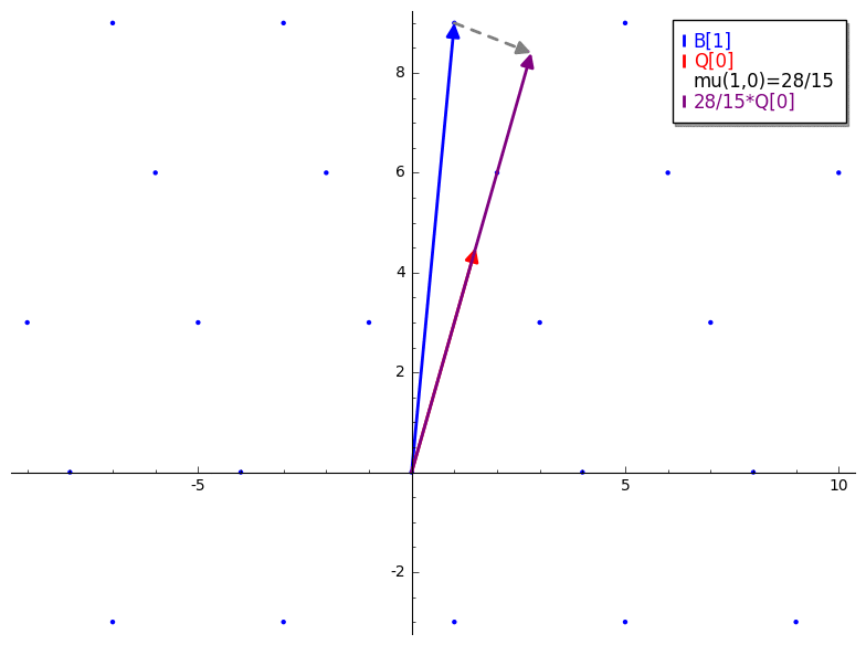
We already know that just applying GS won't necessarily give us a basis for our lattice, but it does give us the “ideal” orthogonalized matrix. Since we cannot use the “ideal” matrix directly, I like to think of mu as leveraging the GS orthogonalized matrix as a reference to how successful reduction is.

Length Reduction

Isolating the length reduction pseudocode from LLL, we have:

1.  n, k = B.nrows(), 1
2.  # outer loop condition
3.  while k < n:
4.      # length reduction loop
5.      for j in reversed(range(k)):
6.          if abs(mu(k,j)) > .5:
7.              # reduce B[k]
8.              B[k] = B[k] - round(mu(k,j))*B[j]
9.              # re-calculate GS with new basis B
10.              Q = gram_schmidt(B)

At line 1, we establish two variables:

• n: which is a constant that holds the number of rows in the basis B

• k: which keeps track of the index of the vector we are focusing on

The outer loop condition is less of a concern during the length reduction step, we can head straight to the length reduction loop. The length reduction loop iterates through the k-1th basis vector towards the 0th basis vector and checks if the absolute value of mu(k,j) is greater than 1/2. 1/2 is significant for since we are rounding the value of mu(k,j), if its absolute value is less than 1/2 then we would be subtracting a zero vector which wouldn't reduce the vector. We could remove that if statement on line 6 but we would then have superfluous assignments (i.e. B[k] = B[k]) for some iterations.

The length reduction step is basically Gram-Schmidt's reduction step with minor modifications. Here is another way to write the LLL length reduction step (omitting the if condition) for each vector in a length reduction loop:

B[0] = B[0]
B[1] = B[1] - round(mu(1, 0))*B[0]
B[2] = B[2] - round(mu(2, 1))*B[1] - round(mu(2, 0))*B[0]
...
B[k] = B[k] - round(mu(k, k-1))*B[k-1] - round(mu(k, k-2))*B[k-2] - ... - round(mu(k, 0))*B[0]

Just for comparison here is how Gram-Schmidt vectors are calculated:

Q[0] = B[0]
Q[1] = B[1] - mu(1, 0)*Q[0]
Q[2] = B[2] - mu(2, 1)*Q[1] - mu(2, 0)*Q[0]
...
Q[k] = B[k] - mu(k, k-1)*Q[k-1] - mu(k, k-2)*Q[k-2] - ... - mu(k, 0)*Q[0]

And finally, after we modify our basis B, we need to keep our orthogonalized basis up-to-date. In line 10, we update Q. This is definitely not the most efficient way to keep Q up-to-date, but I just copied Wikipedia here so ¯\(ツ)/¯.

The Lovász Condition and the Swap Step

Extracting the “swap” step from our Wikipedia pseudocode gets us:

1.      # swap step
2.      if Q[k]*Q[k] >= (delta - mu(k,k-1)**2)*(Q[k-1]*Q[k-1]):
3.          k = k + 1
4.      else:
5.          B[k], B[k-1] = B[k-1], B[k]
6.          Q = gram_schmidt(B)
7.          k = max(k-1, 1)
8.
9. return B

At this point, the algorithm has finished a round of length-reduction. From there LLL must determine what vector to focus on next. The Lovász condition will tell us whether to continue on to the next basis vector (Line 3), or whether to place the k'th basis vector in position k-1 (Lines 5-7).

Putting the meaning of the Lovász condition aside for now, this swap step is reminiscent of a sorting algorithm. Recall that k is the index of the basis vector that LLL is “focusing on”. Suppose LLL is at the kth vector and the Lovász condition is true, from there LLL just moves onto the k+1th vector (Line 3). At this stage, LLL is basically saying that the 0th to kth vectors are roughly sorted by length (this may change after the next round of reductions though). If the Lovász condition is false, the kth basis vector is placed at position k-1 (Line 5), and LLL then re-focuses (Line 7) on the same vector which is now at position k-1. Another reduction round is done, and then back to the swap step. This brings about another way to describe LLL: LLL is a vector sorting algorithm that occasionally screws up the ordering by making vectors smaller so it has to re-sort.

What about the Lovász condition, itself? As I said earlier, it's basically a heuristic that determines if the vectors are in a “good” order. Aside from that, I don't have too much to add here unfortunately as my intuition is still shaky. There are multiple equivalent representations for the Lovász and none of them have really felt 100% right to me. The best explanations that I have found thus far are this StackOverflow post and “An Introduction to Mathematical Cryptography” .

“An Introduction to Mathmetical Cryptography” discusses an equivalent representation of the Lovász condition that is a comparison of the lengths of the projection of basis vectors onto the orthogonal complement of a space spanned by a subset of basis vectors.

If anyone reading this has a link to a decently intuitive explanation or can describe the Lovász in a memorable way please let me know!

Things that Stumped Me When Learning LLL

Is the Gaussian length-reduction step guaranteed to provide short and nearly orthogonal vectors?

If you have not made the connection yet, the m value from Gaussian reduction is the nearest integer of the mu value from Gram-Schmidt. It may not seem obvious that rounding the result of mu and using as a scalar would produce a good basis. In Gram-Schmidt using the exact value of mu allows for the ideal decomposition of a vector, which can be used to orthogonalize the vector in relation to the other basis vectors. With Gaussian reduction, we are rounding that result which could affect the orthogonality. Fortunately, even after rounding mu the length reduction step will produce “nearly orthogonal” vectors.

In fact, a new length-reduced vector B[k] where B[k] = B[k] - round(mu(i,j))*B[j] will always have an angle with B[j] that lies between 60 and 120 degrees. This is guarantee that stems from another fact that B[k]'s projection onto B[j] will always lie between -1/2*B[j] and 1/2B[j]. Why is the latter fact true? Intuitively, we have removed all possible integer components of B[j] from B[k], therefore, the resultant projection of B[k] onto B[j] must lie between -1/2*B[j] and 1/2B[j].

Suppose we have just reduced B[k], so we know the projection of B[k] onto B[j] will lie between -1/2*B[j] and 1/2*B[j]. Using the definition of vector projection (see image below), we can re-write our inequality:

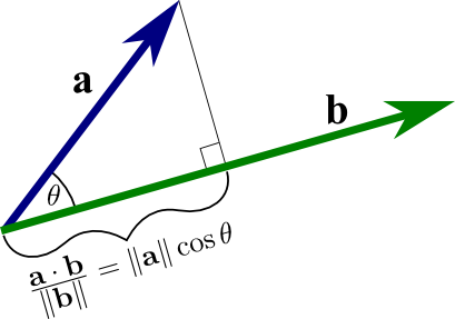
|B[k]|*cos(theta) = proj B[k] onto B[j]
=>
|B[k]|*abs(cos(theta)) <= 1/2*|B[j]|
(|B[k]|/|B[j]|)*abs(cos(theta)) <= 1/2

I alluded to this earlier, but Gaussian two dimensional reduction will make it such that the reduced vector B[k] is shorter than B[j] (there is a proof of this in “Introduction to Mathematical Cryptography”). According to this StackOverflow post , these two facts prove the “nearly” orthogonal property of the output vectors. I am actually not 100% sure these proofs are correct (I think they made a mistake but I don't have a proof either) so I cannot say much more than that.

Why doesn't Gaussian lattice reduction easily generalize to work with lattices with more than 2 vectors?

I found the explanation from “Mathematics of Public Key Cryptography” to explain this well.

Finally, we remark that there is a natural analogue of Gaussian Reduction for any dimension. Hence, it is natural to try to generalise the Lagrange-Gauss algorithm to higher dimensions. Generalisations to dimension three have been given by Vall'ee and Semaev. Generalising to higher dimensions introduces problems. For example, choosing the right linear combination to size reduce bn using b1,…,bn−1 is solving the CVP in a sublattice (which is a hard problem). Furthermore, there is no guarantee that the resulting basis actually has good properties in high dimension. We refer to Nguyen and Stehl'e for a full discussion of these issues and an algorithm that works in dimensions 3 and 4

How does LLL overcome this? I like to think that LLL breaks an n-dimensional problem down into a bunch of 2-dimensional cases and works a little at a time. That technique, plus length-sorting approximations, seems to work well in practice.

How does LLL use GS as a guide?

Again, quoting others that are smarter than I am:

As we have noted in Example 16.3.3, computational problems in lattices can be easy if one has a basis that is orthogonal, or “sufficiently close to orthogonal”. A simple but important observation is that one can determine when a basis is close to orthogonal by considering the lengths of the Gram-Schmidt vectors. More precisely, a lattice basis is “close to orthogonal” if the lengths of the Gram-Schmidt vectors do not decrease too rapidly.

Thanks to Chris Bellavia for providing valuable feedback on this write-up.